4.3.2. Non-Linear least squares
Contents
Where not otherwise denoted, the main sources are [IMM3215] and wikipedia.
Let  be a function of
  with parameters
  .
Unlike Generalized linear models, the function
.
Unlike Generalized linear models, the function  may be
nonlinear in the parameters , for example
may be
nonlinear in the parameters , for example
![M_\theta(x) = \theta_0 \exp(\theta_1 x) + \theta_2 \exp(\theta_3 x)
\quad \text{with} \, \theta = [ \theta_0, \theta_1, \theta_2, \theta_3 ]^T](_images/math/52a3be2687acab205bfa99a4ac4ca7098dbb6e35.png)
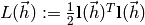
The aim of non-linear least squares is to find the parameters such that
the function fits a set of training data (input and output values of )
optimally with respect to the sum of squares residual.
The input and output values  can be considered to be constant, as the
minimization is over the function parameters . To make the notation
simpler, the functions
can be considered to be constant, as the
minimization is over the function parameters . To make the notation
simpler, the functions  are further defined as:
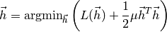
and the optimization problem can therefore be reformulated:
Note
In contrast to Generalized linear models, the presented algorithms only
find local minimal. A local minima of a function  is defined by the
following equation, given a (small) region
is defined by the
following equation, given a (small) region  :
:

4.3.2.1. Gradient descent methods
Descent methods iteratively compute the set  from a prior
set
from a prior
set  by
by
with the initial set  given. The moving direction
  and step size
  have to be determined in such a way that the step
was actually a descent, i.e. the following equation holds for each step
have to be determined in such a way that the step
was actually a descent, i.e. the following equation holds for each step  :
:
The step size can be set to a constant, e.g.  or
determined by Line search (or another method). A constant value is
justified as the line search algorithm may take a lot of time.
or
determined by Line search (or another method). A constant value is
justified as the line search algorithm may take a lot of time.
4.3.2.1.1. Steepest descent
Let  be the gradient of
  .
.
![\nabla(\theta) := \left[ \frac{\partial F(\theta) }{ \partial \theta_0 }, \frac{\partial F(\theta) }{ \partial \theta_1 },
\dots, \frac{\partial F(\theta) }{ \partial \theta_n } \right]^T](_images/math/24b80fb881f6616751b76583c4c66677f1d45392.png)
The gradient can be seen as the direction of the steepest increase
in the function . Hence, the steepest descent method or also named gradient method
uses its negative as moving direction  .
.
The choice of the gradient is reasonable, as it is locally the best choice since the descent is maximal.
This method converges but convergence is only linear, thus it is often used if is
still far from the minimum  .
.
The steepest descent algorithm can be summarized as follows:
Init
 .
.- Iterate
- .
- Compute (using Line search or another method).
 .
.- Stop, if is small enough.
4.3.2.1.2. Newton’s method
Let  be the Hessian matrix of
![\mathbf{H}(\theta) = \left[ \frac{ \partial^2 F(\theta) }{ \partial \theta_i \, \partial \theta_j } \right]](_images/math/bf72ecf12667304e3ac315ec885a27c34165a050.png)
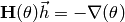
As is an extremal point, the gradient must be zero  .
Thus, is a stationary point of the gradient. Using a second order Taylor
expansion of the gradient around , one gets the equation
.
Thus, is a stationary point of the gradient. Using a second order Taylor
expansion of the gradient around , one gets the equation
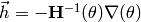
Setting  yields the moving direction of Newton’s method:
The algorithm can be defined analogous to the Steepest descent algorithm.
Init
.- Iterate
- Solve
 .
. - Compute (using Line search or another method).
- .
- Stop, if is small enough.
- Solve
Newton’s method has up to quadratic convergence but may converge to a maximum.
Thus it is only appropriate, if the estimate is already close to the
minimizer . A big problem with Newton’s method is that the second derivative
is required, a prerequisite that can often not be fulfilled.
To combine the strengths of both methods, a hybrid algorithm can be defined
Init
.- Iterate
- If is positive definite, Newton’s method is used:
 .
. - Otherwise, the gradient method is applied:
.
- Compute (using Line search or another method).
- .
- Stop, if is small enough.
- If
4.3.2.1.3. Line search
All above algorithms require a computation of the step size . The
line search algorithm either computes the optimal or an estimate step size when
the current estimate and moving direction are given.
Let’s consider the function
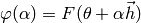
The goal is to find the step size that minimizes the above function. If
is too low, it should be increased in order to speed up convergence. If it is to high,
the error might not decrease (if  has a minimum), thus has to be decreased.
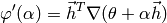
A nice property of this function is that its derivation can easily be seen to be
The exact line search algorithm aims to find a good approximation of the minimum
whereas the soft line search method only ensures that the  is within
some boundary. The soft line search algorithm is often preferred, as it is usually
faster and a close approximation to the minimum is not required.
is within
some boundary. The soft line search algorithm is often preferred, as it is usually
faster and a close approximation to the minimum is not required.
The soft line search uses the two following constraints for  :
:
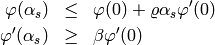
with  and
and  . The first
constraint ensures that the error decreases, the second one inhibits that
the decrease is too small.
. The first
constraint ensures that the error decreases, the second one inhibits that
the decrease is too small.
The line search algorithm comes from the idea to construct an interval ![[a,b]](_images/math/8ecbd1ba3da8f2adef66a63f2ab32c47e63fa734.png) which defines the range of acceptable values for and successively
narrow down this interval.
which defines the range of acceptable values for and successively
narrow down this interval.
Let’s define 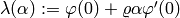 , the
right hand side of the first constraint.
, the
right hand side of the first constraint.  is a parameter
that inhibits the right side of the interval
is a parameter
that inhibits the right side of the interval  to become arbitrary large, in
the case of being unbounded.
to become arbitrary large, in
the case of being unbounded.
Initialize

Initialize
- Iterate while
 and
and  and
and 
- Iterate while

- Iterate while
 or
or 
- Refine

- Refine
- Iterate while

The first iteration shifts the initial interval to the right as long as the second
constraint is not fulfilled. The second iteration shrinks the interval until a solution
for is found for which both constraints hold. The refinement routine is defined as:
- Initialize

- Initialize
- If
 , set
, set 
- Otherwise, set

- If
 , set
, set 
- Otherwise, set

The first branching adjusts the by approximating  with
a second order polynomial. If the approximation has a minimum, it is taken, otherwise
is set to the midpoint of the interval . In the first
case, it is made sure that the interval decreases by at least 10%. The second
branching reduces the interval, such that the new interval still contains acceptable
points.
with
a second order polynomial. If the approximation has a minimum, it is taken, otherwise
is set to the midpoint of the interval . In the first
case, it is made sure that the interval decreases by at least 10%. The second
branching reduces the interval, such that the new interval still contains acceptable
points.
The difference between soft line search and exact line search is the second iteration in the algorithm. For the exact line search, line (5) becomes
- Iterate while
 and
and 
- Refine
- Refine
- Iterate while
with  being error tolerance parameters. [IMM3217]
4.3.2.2. Gauss-Newton algorithm
Let  be the number of samples and the number of parameters.
Note that
be the number of samples and the number of parameters.
Note that ![\mathbf{f}(\theta) := \left[ f_0(\theta), f_1(\theta), \dots, f_{n-1}(\theta) \right]^T](_images/math/34657ee0a6372639b01ee819ad939b5fbcda2395.png) is defined. Furthermore, the
is defined. Furthermore, the  Jacobian matrix is
![\mathbf{J}(\theta)_{ij} = \left[ \, \frac{\partial f_i(\theta) }{ \partial \theta_j} \, \right]](_images/math/5920da42d30eb0f94b678f0a014d4f87654a4846.png)
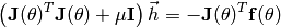
The Gauss-Newton algorithm approximates the function  using a second order taylor expansion
  around .
This then is used to formulate the minimization problem
around .
This then is used to formulate the minimization problem
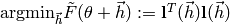 which is equivalent to solving the linear equation
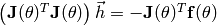 .
As in Newton’s method, the rationale behind this is that the minimum of the
approximation can actually be computed. While Newton’s method minimizes the
approximated gradient
.
As in Newton’s method, the rationale behind this is that the minimum of the
approximation can actually be computed. While Newton’s method minimizes the
approximated gradient  , the Gauss-Newton algorithm approximates the function
 directly.
Init
.- Iterate
- Solve
 .
. - Compute (using Line search or another method).
- .
- Stop, if is small enough.
- Solve
The algorithm converges, if  has full rank in all
iteration steps and if is close enough to . This
implies that the choice of the initial parameters not only influences the result
(which local minima is found) but also convergence.
For close to , convergence becomes quadratic.
has full rank in all
iteration steps and if is close enough to . This
implies that the choice of the initial parameters not only influences the result
(which local minima is found) but also convergence.
For close to , convergence becomes quadratic.
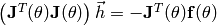
The algorithm can be easily be extended to handle sample weights. Let  be the matrix with the weights in its diagonal
  . Then, the
linear equation to be solved in the iteration step (1) becomes
. Then, the
linear equation to be solved in the iteration step (1) becomes
4.3.2.3. Levenberg-Marquardt algorithm
The Levenberg-Marquardt algorithm introduces a damping parameter  to
the Gauss-Newton algorithm. Using
to
the Gauss-Newton algorithm. Using
 ,
the minimization problem is reformulated as
,
the minimization problem is reformulated as
and can be computed by solving by the linear equation
From the first equation, it can be seen that the damping parameter adds a penalty
proportional to the length of the step . Therefore, the step size
can be controlled by  which makes the step size parameter obsolete.
The damping parameter
which makes the step size parameter obsolete.
The damping parameter  can intuitively be described by the following two cases:
- is large. The linear equation is approximately
 , thus
 equivalent to the Steepest descent method with small step size.
- is small (zero in the extreme). The optimization problem becomes more
similar to the original one. This is desired in the final state, when
is close to .
Like in Line search, the damping parameter can be adjusted iteratively. The gain ratio calculates the ratio between the actual and predicted decrease and is defined as
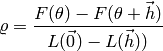
where  is a second order Taylor expansion of around .
The denominator can be seen to be
is a second order Taylor expansion of around .
The denominator can be seen to be  .
Using this, the damping parameter is set in each step according to the following routine (according to Nielsen):
.
Using this, the damping parameter is set in each step according to the following routine (according to Nielsen):
- If

 .
.
- If
- Otherwise


with , initially. The gain ratio is negative if the step
does not actually decrease the target function . If the gain ratio is below
zero as in step (2), the current estimate of is not updated.
The written-out Levenberg-Marquardt algorithm with adaptive damping parameter looks like this:
Initialize
Initialize
Initialize
![\mu = \tau \max\limits_i \left[ \mathbf{J}(\theta_0)^T \mathbf{J}(\theta_0) \right]_{ii}](_images/math/f160c7df68135d52964b73d31b101068e89a06a0.png)
- Iterate
- Solve
 .
. - Compute the gain ratio.
- If the gain ratio is positive, compute
 and update the parameter estimate
- Otherwise adjust
- Stop, if the change in or the gradient is small enough.
- Solve
 and are parameters of the algorithm and therefore have to be
provided by the user. The algorithm could also be formulated like the
Gauss-Newton algorithm with a constant dumping parameter.
Yet, this would do not much more than introduce an additional parameter, thus won’t
be benefitial.
and are parameters of the algorithm and therefore have to be
provided by the user. The algorithm could also be formulated like the
Gauss-Newton algorithm with a constant dumping parameter.
Yet, this would do not much more than introduce an additional parameter, thus won’t
be benefitial.
Like in the Gauss-Newton algorithm, the optimization problem can also incorporate sample weights:

4.3.2.4. Interfaces
- class ailib.fitting.NLSQ(model, derivs, initial=None, lsParams=None, sndDerivs=None)
Non-linear least-squares base class.
This is an incomplete class for nonlinear least-squares algorithms. The class provides some basic routines that are commonly used.
Subclasses are required to write the coeff member after fitting. Otherwise some routine calls may fail or produce wrong results. The default strategy for the step size is a constant.
Warning
Local minima!
Throughout the documentation of this class, the following type symbols are used: - a: The parameters of the model. ???????? - b: The input of the model. May be arbitrary. - c: The output of the model. ????????? - N: Number of training samples. - M: Number of model function parameters.
The search line parameters are: - rho ? - beta ? - al_max ? - tau ? - eps ?
Warning
parameter dependence!
Parameters: - model ((Num c) :: a -> b -> c) – Model function to be fitted.
- derivs ([(Num c) :: a -> b -> c]) – First order derivations of the model function. Expected is list where the i’th element represents the derivation w.r.t the i’th parameter.
- initial (c) – Initial choice of parameters. The initial choice may influence result and convergence speed.
- lsParams ([float]) – Line search parameters
- sndDerivs ([[(Num c) :: a -> b -> c]]) – Second order partial derivations of the model function. Expected is a matrix of functions where the element (ij) represents the derivations w.r.t the i’th first and then the j’th parameter. Only required for the Hessian matrix.
- err((x, y))
- Squared residual.
- eval(x)
- Evaluate the model at data point x with coefficients after fitting.
- fit(features, labels=None, weights=None)
Fit the model to the training data.
Parameters: - features – Training samples.
- labels – Target values.
- weights ([float]) – Sample weights.
Returns: self
- grad(theta, data)
Compute the Gradient of the error function.
The error function is dependent on the model function parameters and the training data. This information has to be provided.
Todo
Cannot handle weights. Implemented but commented out (not tested, not quite sure)
Parameters: - theta (a) – The parameters of the model function.
- data (STD) – The training samples.
Returns: Gradient as a (Nx1) matrix
- hessian(theta, data)
Compute the Hessian matrix of the error function.
In order to compute the hessian, the first and second order partial derivatives have to be specified (use the constructor’s sndDerivs parameter). The error function is dependent on the model function parameters and the training data. This information has to be provided.
Todo
Cannot handle weights. Implemented but commented out (not tested, not quite sure)
Parameters: - theta (a) – The parameters of the model function.
- data (STD) – The training samples.
Returns: Hessian matrix (MxM)
- jacobian(theta, data)
Compute the Jacobian matrix of the error function.
The error function is dependent on the model function parameters and the training data. This information has to be provided.
Todo
Cannot handle weights. Actually, as J_ij = [df<j>/dt<i>], weights don’t appear In the context of Gauss-Newton and Levenberg-Marquandt, J*W is used.
Parameters: - theta (a) – The parameters of the model function
- data (STD) – The training samples.
Returns: Jacobian matrix (NxM)
- class ailib.fitting.SteepestDescent(model, derivs, initial=None, eps=0.001, maxIter=100, lsParams=None)
Bases: ailib.fitting.nlsq.NLSQ
Implementation of the Steepest descent algorithm.
The initial parameter values and convergence threshold have to be set either at object construction or at the call to the fit method. The latter overwrites the former.
The default strategy for step size computation is the Soft line search. This behaviour can be modified through the alpha member. Example:
>>> o = SteepestDescent(...)
>>> o.alpha = o._exactLineSearch
If the fitting fails due to an OverflowError, try modifying the line search parameters. Consider setting al_max to a relatively small value (<< 1.0), although this will increase convergence time.
Parameters: - model ((Num c) :: a -> b -> c) – Model function to be fitted.
- derivs ([(Num c) :: a -> b -> c]) – First order derivations of the model function. Expected is list where the i’th element represents the derivation w.r.t the i’th parameter.
- initial (c) – Initial choice of parameters. The initial choice may influence result and convergence speed.
- eps (float) – Convergence threshold. The iteration stops, if the step length is below this threshold.
- maxIter (int) – Maximum number of iterations.
- lsParams ([float]) – Line search parameters.
- fit(samples, labels, weights=None, theta=None, eps=None)
Determine the parameters of a model, s.t. it optimally fits the training data.
The parameters theta and eps are optional. If one of the is not set, its default value determined at object construction will be used (use the constructor’s initial and eps arguments).
Parameters: - samples ([]) – Training data.
- labels ([]) – Training labels.
- weights ([float]) – Sample weights.
- theta (a) – Initial parameter choice.
- eps (float) – Convergence threshold. The iteration stops, if the step length is below this threshold.
Returns: self
- class ailib.fitting.Newton(model, derivs, sndDerivs, initial=None, eps=None, maxIter=100, lsParams=None)
Bases: ailib.fitting.nlsq.NLSQ
Implementation of Newton’s method.
Parameter handling and step size strategy behave as in SteepestDescent
Parameters: - model ((Num c) :: a -> b -> c) – Model function to be fitted.
- derivs ([(Num c) :: a -> b -> c]) – First order derivations of the model function. Expected is list where the i’th element represents the derivation w.r.t the i’th parameter.
- sndDerivs ([[(Num c) :: a -> b -> c]]) – Second order partial derivations of the model function.
- initial (c) – Initial choice of parameters. The initial choice may influence result and convergence speed.
- eps (float) – Convergence threshold. The iteration stops, if the step length is below this threshold.
- maxIter (int) – Maximum number of iterations.
- lsParams ([float]) – Line search parameters
- fit(samples, labels, weights=None, theta=None, eps=None)
Determine the parameters of a model, s.t. it optimally fits the training data.
The parameters theta and eps are optional. If one of the is not set, its default value determined at object construction will be used (use the constructor’s initial and eps arguments).
Parameters: - samples ([]) – Training data.
- labels ([]) – Training labels.
- weights ([float]) – Sample weights.
- theta (a) – Initial parameter choice.
- eps (float) – Convergence threshold. The iteration stops, if the step length is below this threshold.
Returns: self
- class ailib.fitting.HybridSDN(model, derivs, sndDerivs, initial=None, eps=None, maxIter=100, lsDescent=None, lsNewton=None)
Bases: ailib.fitting.nlsq.Newton
Implementation of the Hybrid SD/Newton algorithm.
The Newton step is chosen, if the Hessian matrix is positive definite. Otherwise, the steepest descent method is applied.
Parameter handling and step size strategy behave as in SteepestDescent
Parameters: - model ((Num c) :: a -> b -> c) – Model function to be fitted.
- derivs ([(Num c) :: a -> b -> c]) – First order derivations of the model function. Expected is list where the i’th element represents the derivation w.r.t the i’th parameter.
- sndDerivs ([[(Num c) :: a -> b -> c]]) – Second order partial derivations of the model function.
- initial (c) – Initial choice of parameters. The initial choice may influence result and convergence speed.
- eps (float) – Convergence threshold. The iteration stops, if the step length is below this threshold.
- maxIter (int) – Maximum number of iterations.
- lsDescent ([float]) – Line search parameters for the steepest descent part.
- lsNewton ([float]) – Line search parameters for the newton part.
- fit(samples, labels, weights=None, theta=None, eps=None)
Determine the parameters of a model, s.t. it optimally fits the training data.
The parameters theta and eps are optional. If one of the is not set, its default value determined at object construction will be used (use the constructor’s initial and eps arguments).
Parameters: - samples ([]) – Training data.
- labels ([]) – Training labels.
- weights ([float]) – Sample weights.
- theta (a) – Initial parameter choice.
- eps (float) – Convergence threshold. The iteration stops, if the step length is below this threshold.
Returns: self
- class ailib.fitting.GaussNewton(model, derivs, initial=None, eps=None, maxIter=100, lsParams=None)
Bases: ailib.fitting.nlsq.NLSQ
Implementation of the Gauss-Newton algorithm.
Parameter handling and step size strategy behave as in SteepestDescent
Parameters: - model ((Num c) :: a -> b -> c) – Model function to be fitted.
- derivs ([(Num c) :: a -> b -> c]) – First order derivations of the model function. Expected is list where the i’th element represents the derivation w.r.t the i’th parameter.
- initial (c) – Initial choice of parameters. The initial choice may influence result and convergence speed.
- eps (float) – Convergence threshold. The iteration stops, if the step length is below this threshold.
- maxIter (int) – Maximum number of iterations.
- lsParams ([float]) – Line search parameters
- fit(samples, labels, weights=None, theta=None, eps=None)
Determine the parameters of a model, s.t. it optimally fits the training data.
The parameters theta and eps are optional. If one of the is not set, its default value determined at object construction will be used (use the constructor’s initial and eps arguments).
Parameters: - samples ([]) – Training data.
- labels ([]) – Training labels.
- weights ([float]) – Sample weights.
- theta (a) – Initial parameter choice.
- eps (float) – Convergence threshold. The iteration stops, if the step length is below this threshold.
Returns: self
- class ailib.fitting.Marquardt(model, derivs, initial=None, eps0=0.01, eps1=0.01, tau=1.0, maxIter=100)
Bases: ailib.fitting.nlsq.NLSQ
Implementation of the Levenberg-Marquardt algorithm.
The damping parameter
is initialized with tau and adjusted
according to Nielsen’s strategy.Parameters: - model ((Num c) :: a -> b -> c) – Model function to be fitted.
- derivs ([(Num c) :: a -> b -> c]) – First order derivations of the model function. Expected is list where the i’th element represents the derivation w.r.t the i’th parameter.
- initial (c) – Initial choice of parameters. The initial choice may influence result and convergence speed.
- eps0 (float) – Convergence threshold. The iteration stops, if the maximal gradient component is below this threshold.
- eps1 (float) – Convergence threshold. The iteration stops, if the relative change in the model parameters is below this threshold.
- tau (float) – Constant for determining the initial damping. Use a small value (10**(-6)), if the initial parameters are believed to be a good approximation, otherwise use 10**(-3) or 1.0 (default)
- maxIter (int) – Maximum number of iterations.
- fit(samples, labels, weights=None, theta=None, eps0=None, eps1=None, tau=None)
Determine the parameters of a model, s.t. it optimally fits the training data.
The parameters theta, eps0, eps1 and tau are optional. If one of the is not set, its default value determined at object construction will be used (use the constructor’s initial, eps0, eps1 and tau arguments).
Parameters: - samples ([]) – Training data.
- labels ([]) – Training labels.
- weights ([float]) – Sample weights.
- theta (a) – Initial parameter choice.
- eps0 (float) – Convergence threshold. The iteration stops, if the maximal gradient component is below this threshold.
- eps1 (float) – Convergence threshold. The iteration stops, if the relative change in the model parameters is below this threshold.
- tau (float) – Constant for determining the initial damping. Use a small value (10**-6), if the initial parameters are believed to be a good approximation, otherwise use 10^-3 or 1.0 (default)
Returns: self