1. Introduction
Contents
1.1. About this library
This library provides several algorithms from the field of machine learning and statistics. A short introduction into statistics is given in the next chapter. The goal of this documentation is to provide a theoretical background additional to the implementation. Main topics covered so far are sampling methods, model fitting and model selection. The model fitting module provides various many different learning algorithms. Where possible, it was tried to stick to a statistics and information theory framework.
Besides the python standard library, the framework mainly uses scipy and numpy. Although not all algorithms rely on them, it’s strongly encouraged to use those libraries.
Other projects that might be useful in what you try to achieve can be found at scikit. Especially noteworthy is the package scikit-learn that covers a lot of machine learning algorithms. For statistical computation, there’s a nice list of projects as StatPy. Noteworthy are also the SciTools package, the MatPlotLib for plotting and the convex optimization package cvxopt.
If you’re looking for more theoretical information, note the used Resources. On the web, many topics are well covered by wikipedia and also the StatSoft Statistics textbook might be useful.
1.1.1. Type notations
It’s important to understand the type signatures. It may help a lot to understand the structure of the code.
Wherever a common type like float or int (or a type that mimics it) is expected, this is noted using the python syntax. Where a list is expected, also the respective python symbol is used. For exampe, [[float]] would be a matrix of floats whereas (float) is a tuple of floats. Lists and tuples are usually exchangable but it’s strongly recommended to use the specified one. The syntax for functions and unspecified types is haskell-like. If the there are no restriction on a type, a character is paced instead. Several types are concatenated using an arrow (->) and the last type in the chain is the return value. Consider the example below:
>>> (Num b) :: [a] -> b -> a
This signature defines a function that takes a list of an arbitrary type and a second parameter of (possibly) another type and returns a value of the same type as the first parameter’s list type. Additionally, if a type is requested to behave like a nummerical type (int or float), this is indicated as above for the type b. Several restrictions are seperated by comma. Besides the nummerical restriction, also Ord (orderd type) may appear. A function with this signature could be as simple as
>>> lambda lst,idx: lst[idx]
Usually, the type symbols are coherent within all methods of a class and often also with related classes (i.e. classes in the same document).
If no type signature is given, the type is completely arbitrary. However, note that this is usually the case for abstract methods and type restrictions may be found in their concrete implementations.
1.2. Statistics formulary
1.2.1. Combinatorics
Draws of objects from an urn. There are n objects and k draws.
| Ordered | Unordered | |
| With replacement | n^k | (n+k-1)!/((n-1)!*k!) |
| Without replacement | n!/(n-k)! | n!/((n-k)!*k!) |
1.2.2. Random variables and probability mass function
Consider an experiment with several possible outcomes where the outcome depends on some underlying random
process. A prominent example is a coin toss where the possible results are head and tail.
The set of all the experiment’s outcomes is the sample space  .
Depending on the nature of the experiment, it may be either discrete or continous.
.
Depending on the nature of the experiment, it may be either discrete or continous.
Such an experiment can be expressed through a random variable  .
A random variable can be viewed as a function that assigns a value (often a real number) to any
element of the sample space .
.
A random variable can be viewed as a function that assigns a value (often a real number) to any
element of the sample space .

If the sample space is continous, then so is the random
variable . If is countable, then is discrete. Note that for
the space of a variable, always the calligraphic sign (e.g.  )
is used.
)
is used.
The probability mass function ![P: \mathcal{A} \rightarrow [0,1]](_images/math/6708389b7fb476c346020ef3f16b705befc60e67.png) gives the probability of
seeing a specific outcome of a random variable. If the random variable is continous, this probability has
to be zero, so
gives the probability of
seeing a specific outcome of a random variable. If the random variable is continous, this probability has
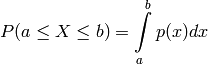
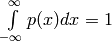
to be zero, so  . The probability of seeing any possible outcome must be one, hence
Usually, the random variable is denoted with an uppercase letter () whereas a lower case letter ( ) is
used for a specific value of the variable. Also, in order to make mathematical terms more readable, the following
notation is used:
) is
used for a specific value of the variable. Also, in order to make mathematical terms more readable, the following
notation is used:
Given two random variables  , the probability that the respective outcomes are and
 are observed at the same time is called the joint probability
  .
.
Two random variables are independent, if and only if
holds. Independence means that the outcome of one random variable does not influence the outcome of the other one.
If two random variables are independent, one can easily find the probability of one of the two variables by summing
or integration over the other one, i.e. 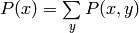 if the variables are discrete.
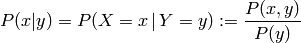
The conditional probability  is the probability of seeing a certain outcome ,
given that the outcome of the other random variable was already observed to be .
is the probability of seeing a certain outcome ,
given that the outcome of the other random variable was already observed to be .
For independent variables, it can be seen that 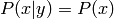 , which intuitively makes sense as
doesn’t influence .
, which intuitively makes sense as
doesn’t influence .
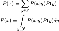
The law of total probability, also called marginalization, states the following:
1.2.3. Bayes
The Bayes theorem states the following:
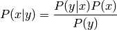
The term  is the prior probability, as its independent of and can thus be interpreted
as the probability of an outcome of where no information about the second variable
is the prior probability, as its independent of and can thus be interpreted
as the probability of an outcome of where no information about the second variable  is available.
In this view, the conditional probability is the posterior, so the probability after some information
was already observed. The denominator
is available.
In this view, the conditional probability is the posterior, so the probability after some information
was already observed. The denominator  is for normalization, hence also called normalizer.
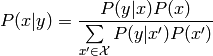
Using the law of total probability, the theorem can be re-written into the following form:
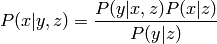
If there are three random variables, the probability of the outcome , given that the two outcomes
 are observed is
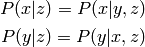
Two variables are conditionally independent, iff

given a third random variable  . It follows that
In robotics, the term Belief is sometime used. Let  be a sequence
of measurements
be a sequence
of measurements  and actions
  up to time
  . The
belief expressed the probability of being in the current state
. The
belief expressed the probability of being in the current state  :
:

1.2.4. Probability distributions
The term probability distribution is used to describe the collection of the probabilities for all possible outcomes. When talking about a probability distribution, usally the probability mass or density functions are referred to.
Remember the probability mass function (pmf)  , already defined above. It expresses how
probable a certain outcome is and it holds that
, already defined above. It expresses how
probable a certain outcome is and it holds that
In the discrete case, also the probability of several outcomes can be computed easily by
For discrete  , the probability of any element is non-negative and strictly
positive for at least one
, the probability of any element is non-negative and strictly
positive for at least one  . On the other hand, if
is continous, the probability of one exact value goes to zero, hence
. On the other hand, if
is continous, the probability of one exact value goes to zero, hence  .
In consequence, for continous functions we define
.
In consequence, for continous functions we define
with  the probability density function (pdf). Analogous to the pmf, the
probability density function describes how likely a certain outcome is for the
random varaible. The pdf is also non-negative all probabilities sums up to one,
the probability density function (pdf). Analogous to the pmf, the
probability density function describes how likely a certain outcome is for the
random varaible. The pdf is also non-negative all probabilities sums up to one,
 .
.
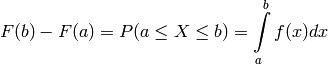
Further, we can define the cumulative distribution function (cdf):
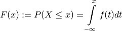
which expresses the probability that the outcome of the experiment will be no larger than .
Note the limits 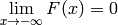 and
and 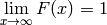 .
From this definition, it’s easily seen that
.
From this definition, it’s easily seen that
If isn’t continous at all places , the probability at the discontinuity is
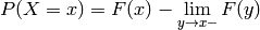
which of course again goes to zero if is continuous at .
For sampling, the inverse cdf would be important. Unfortunately, a closed form representation is often not available. The inverse cdf is defined as
![F^{-1}(y) := \inf\limits_{x} F(x) \geq y \qquad y \in [0,1]](_images/math/4e47c802df8033133d15ae94f0080ebcc2efca57.png)
In other words this means that for a given , find the value
such that  .
.
There are several well known distributions defined in the section Distribution Wrappers and also in the scipy library.
1.2.5. Statistics
Consider a set of data points. Likely, one wants to give some quantitative description of their shape. Also, one would like to be able to give some characterisations of known and well defined probability distributions.
For this, let’s first define the Moment
![\mu_k := E[ X^k ]](_images/math/0fd09118dbe9276900e240fbaf33927335c749ba.png)
using the definition of the Expected value (for discrete and continous random variables)
![E[X] = \sum\limits_{x} x P(x)
E[X] = \int\limits_{x} x f(x) dx](_images/math/964c248bf5ed026d77e796e171fcccac8e79c2f9.png)
Note that  is the probability density function of . The expected value is sometimes referenced as mean
and misleadingly associated with the arithmetic mean. Of course this is only true, if the probability of the observations
is uniform (all observations are equally likely) which is often the case for measured data (then the probability distribution
is expressed by repetition of measurements).
is the probability density function of . The expected value is sometimes referenced as mean
and misleadingly associated with the arithmetic mean. Of course this is only true, if the probability of the observations
is uniform (all observations are equally likely) which is often the case for measured data (then the probability distribution
is expressed by repetition of measurements).
The expected value is linear, a fact that is formally noted by the following equation:
![E[aX + bY + c] = a \, E[X] + b \, E[Y] + c](_images/math/69472b7fec1dcf1957c24aebef6b9b6dfe17e5e1.png)
If the two random variables are independent, it also holds that
![E[X \, Y] = E[X] \, E[Y]](_images/math/b63a3948cb93e8015fff39c48cecafb71c8ef260.png)
The Central Moment is the moment about the expected value, thus
![\mu_k := E[ (X-E[X])^k ]](_images/math/9425e9d7ba0167a3f3473d7ddd2cdc8aac144625.png)
From its definition, one can easily see that the zero’th central moment is one and the first central moment is zero.

The second central moment is the Variance
![\begin{eqnarray*}
\text{Var}[X] &:=& E[ (X-E[X])^2 ] \\
& =& \sum\limits_{x} (x-\mu)^2 P(x) \\
& =& \int\limits_{x} (x-\mu)^2 f(x) dx
\end{eqnarray*}](_images/math/a0294cd06cc59e89abda8d33cac8dd678455cd83.png)
again is the probability density function and ![\mu = E[X]](_images/math/00789be79ce68639023cda441cd8b9fa2e7bbed9.png) the expected value.
The equations show the definition for a discrete and continous random variable, respectively.
An alternative and often more appropriate formulation is
the expected value.
The equations show the definition for a discrete and continous random variable, respectively.
An alternative and often more appropriate formulation is
![\text{Var}[X] = E[X^2] - (E[X])^2](_images/math/4b70984cf8b6d6e3dbfc2a41fff5bf457c0acd34.png)
The variance is pseudo-linear, which means the following:
![\text{Var}[aX+b] = a^2 \text{Var}[X]](_images/math/14025225c0b036e7c5319cfe2f78006f43a45851.png)
A generalisation of the variance to multiple random variables yields the Covariance, which is defined analogously
![\text{Cov}[X,Y] = E[ \left( X-E[X] \right) \left( Y-E[Y] \right) ]](_images/math/dd5fb2237a5b96d8a6aa3c3493f15b4e9084e0f4.png)
For the sake of completeness but without further comment, here are some properties of the covariance:
![\begin{eqnarray*}
\text{Cov}[X,X] &=& \text{Var}[X] \\
\text{Cov}[X,Y] &=& E[X \, Y] - E[X] \, E[Y] \\
\text{Cov}[X,Y] &=& \text{Cov}[Y,X] \\
\text{Cov}[aX + b, Y] &=& a \text{Cov}[X,Y] \\
\text{Cov}[X+Y,Z] &=& \text{Cov}[X,Z] + \text{Cov}[Y,Z]
\end{eqnarray*}](_images/math/dea7ecfc165c275032a83dcf53583c5812c4aa59.png)