2. `core` — Core functionality ¶

Contents

core — Core functionality

2.1. Abbreviations ¶

Some list abbreviations:

head = lambda lst: lst[0]
tail = lambda lst: lst[1:]
last = lambda lst: lst[-1]
init = lambda lst: lst[:-1]

And for tuples:

fst = lambda lst: lst[0]
snd = lambda lst: lst[1]

2.2. Basic math ¶

ailib.sign(x)¶

Return -1 if x is smaller than zero. If x is equal to zero, return zero. Return +1 otherwise.

This method implements the sign function, which is defined as

$\text{sign}(x) = \begin{cases} -1 &, x < 0 \\ 0 &, x = 0 \\ +1 &, x > 0 \end{cases}$

Note that the abbreviation sgn is also available:

sgn := sign

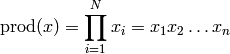
ailib.prod(lst)¶: Return the product of all list elements.

$\text{prod}(x) = \prod\limits_{i=1}^N x_i = x_1 x_2 \dots x_n$

ailib.span(lst)¶: Return the span of a list.

$\text{span}(x) = \max(x) - \min(x)$

ailib.argmin(f, arg)¶

Return the argument for which the value of a function is minimal.

The function f is evaluated at each element of the argument list arg. The value in arg which returns the lowest value of f is returned.

Parameters:	f ((Ord b) => a -> b) – Function to be evaluated. arg (a) – List of argument values.

>>> l1, l2, f = [4,5,6], [1,2,3], lambda x,y: x**2-y**2
>>> argmin(lambda (x,y): f(x,y), itertools.product(l1, l2))
(4, 3)

$\text{arg}\min\limits_{x \in \mathcal{X}} f(x)$

ailib.argmax(f, arg)¶

Return the argument for which the value of a function is maximal.

The function f is evaluated at each element of the argument list arg. The value in arg which returns the lowest value of f is returned.

Parameters:	f ((Ord b) => a -> b) – Function to be evaluated. arg (a) – List of argument values.

>>> l1, l2, f = [4,5,6], [1,2,3], lambda x,y: x**2-y**2
>>> argmax(lambda (x,y): f(x,y), itertools.product(l1, l2))
(6, 1)

$\text{arg}\max\limits_{x \in \mathcal{X}} f(x)$

ailib.normalize(lst, s=1.0)¶

Return the list, such that the elements sum up to s.

Parameters:	lst – A list of numerals. s – Normalize scale.
Returns:	Scaled list with sum(lst) = nrm

>>> normalize([2.0,4.0, 6.0], 3.0)
[0.5, 1.0, 1.5]

>>> sum(normalize([2.0,4.0, 6.0], 3.0))
3.0

$\vec{x}_n = s \frac{\vec{x}}{\lVert{x}\rVert}$

2.3. Distance measurements ¶

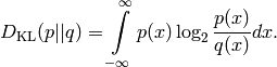
2.3.1. Kullback-Leibler Divergence ¶

The Kullback-Leibler Divergence is defined as:

$D_{\text{KL}}(p || q) = \int\limits_{-\infty}^{\infty} p(x) \log_2 \frac{p(x)}{q(x)} dx.$
ailib.KLD(p, q, r, save=True)¶
Return the continous Kullback-Leibler divergence.

q*(x) must be non-zero for all x in *r. If this doesn’t hold for q, then inf is returned. If the save flag is set, the support r is reduced to the support of q (thus q non-zero for all x in r’).

If you have lists instead of functions, use listFunc() and range().

Parameters:

p ((Num b) :: a -> b) – pdf of the first distribution.

q ((Num b) :: a -> b) – pdf of the second distribution.

r ([a]) – Support.

save (bool) – Flag, if support may be reduced.

Returns:
KLD of p and q, measured at locations in r.
>>> KLD(lambda x: x, lambda x: x-1, [0,1,2,3,4], save=True)
5.4150374992788439
>>> KLD(lambda x: x, lambda x: x-1, [0,1,2,3,4], save=True)
inf

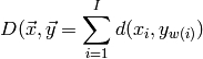
2.3.2. Time warping ¶

Time warping is a distance measurement for two vectors of different size.

ailib.LTW(x, y, dist=<function euclidean at 0x3319500>)¶
Linear time warping.

Parameters:

x ([a]) – First input vector.

y ([b]) – Second input vector.

dist ((Num c) => a -> b -> c) – Distance measurement for vector elements.

Returns:
Linear time warping distance of x, y.
>>> LTW([1,2,3,4,5,6,7], [9,8,7,6])
28.0
Given two input vectors $\vec{x}, \vec{y}$ with lenghts $I,J$ .

$w(i) = \text{Int} \left[ \frac{J-1}{I-1} (i-1) + 1 + 0.5 \right]$

$D(\vec{x}, \vec{y} = \sum\limits_{i=1}^I d(x_i, y_{w(i)})$

2.4. Statistical basics ¶

2.4.1. Average ¶

For all average measurements, the argument lst must be a list of numerics. Note that functions don’t actually need to be implemented as presented here.

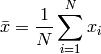
ailib.mean(lst)¶

Return the arithmetic mean of all values of the given list.

$\bar{x} = \frac{1}{N} \sum\limits_{i=1}^N x_i$

ailib.median(lst)¶

Return the median value of the given list.

ailib.gMean(lst)¶

Return the geometric mean of the given values.

$M_g(x) = \sqrt[N]{ \prod\limits_{i=1}^N x_i }$

ailib.hMean(lst)¶

Return the harmonic mean of the given values.

$M_h(x) = \frac{N}{ \sum\limits_{i=1}^N \frac{1}{x_i} }$

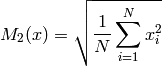
ailib.qMean(lst)¶

Return the quadratic mean of the given values.

$M_2(x) = \sqrt{ \frac{1}{N} \sum\limits_{i=1}^N x_i^2 }$

ailib.cMean(lst)¶

Return the cubic mean of the given values.

$M_3(x) = \sqrt[3]{ \frac{1}{N} \sum\limits_{i=1}^N x_i^3 }$
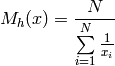
ailib.genMean(lst, p)¶
Return the generalized mean of the given values.

The generalized mean with exponent p is defined as follows:

$M_p(x) = \sqrt[p]{\frac{1}{N} \sum\limits_{i=1}^N x_i^p}$

From this, one can clearly see the following equivalences:
mean = genMean(lst, 1.0)
qMean = genMean(lst, 2.0)
cMean = genMean(lst, 3.0)
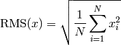
ailib.rms(lst)¶
Return the root mean square of the given values.

$\text{RMS}(x) = \sqrt{ \frac{1}{N} \sum\limits_{i=1}^N x_i^2 }$
>>> rms = qMean
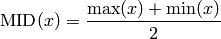
ailib.midrange(lst)¶

Return the midrange of the given values.

$\text{MID}(x) = \frac{\max(x) + \min(x)}{2}$

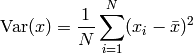
ailib.var(lst)¶

Return the variance of the given list.

Generally, the variance is defined as:

$\text{Var}(x) = E[(X-\mu)^2] = E[X^2] - (E[X])^2$

Here, it is implemented using the arithmetic mean:

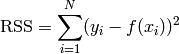
$\text{Var}(x) = \frac{1}{N} \sum\limits_{i=1}^N (x_i - \bar{x})^2$

ailib.rss(lst)¶

Return the residual sum of squares.

The list items are expected to be of the form (f(x),y).

$\text{RSS} = \sum\limits_{i=1}^N ( y_i - f(x_i) )^2$

ailib.binning(data, numBins, hist=False)¶

Divide a list into multiple bins of equal intervalls.

For the type a there must be a float representation and it must be ordered. Specifically, the type must support the functions min, max and float.

Parameters:	data ([a]) – Input list. numBins (int) – Number of bins. hist (bool) – Return the number of samples per bin instead.
Returns:	A list of bins, containing the data elements.

>>> binning([1,2,3,4], 2, hist=False)
[[1,2],[3,4]]

ailib.binRange(data, numBins)¶

Return the intervall boundaries used by binning.

The returned intervalls describe the lower and upper limit, whereas the lower limit is inclusive and the upper limit is inclusive only for the last intervall.

Parameters:	data (a) – Input list. numBins (int) – Number of bins.
Returns:	List of intervalls.

>>> binRange([1,2,3,4], 2, hist=False)
[(1.0,2.5),(2.5,4.0)]

ailib.histogram(data)¶

Count the number of occurrences of tokens in a list.

Parameter:	data – List of tokens.
Returns:	Dict with token as key and relative frequency as value

ailib.majorityVote(data, tieBreaking=<function <lambda> at 0x331da28>)¶

Return the token with the highest number of occurrences.

The tie-breaking rule is applied, if there are several tokens with identical number of occurrences. The tieBreaking function takes two arguments: The tokens with maximal votes and the token histogram. It has to select a single token as a winner. The default function is a random choice.

Parameters:	data (a) – Stream of input tokens. tieBreaking ([a] -> {a -> Int} -> a) – Function to determine the vote winner, in the case of a tie.
Returns:	Token of the data stream with the highest number of occurrences.

>>> majorityVote([1,2,1], tieBreaking=lambda l,h: max(l))
1

>>> majorityVote([1,2,1,2,3], tieBreaking=lambda l,h: max(l))
2

2.5. Distribution Wrappers ¶

So far, no wrapper is fully implemented. Use the distribution related methods of scipy.stats.

2.6. Data conversion ¶

ailib.isList(l)¶: Check, if l is a list type or not.

ailib.listFunc(lst, off=0)¶: Represent a list lst through a function f, such that f(x) = lst [ x + off ].