3. sampling — Sampling Methods
Contents
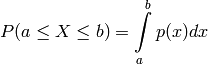
Often, one would like to accquire some samples that follow a certain probability distribution. For example, in algorithm testing, training samples are required but real-world measurements are too rare to be of use, so artificial samples have to be generated. In almost any case, the random samples have to fulfill some constraints, expressed through the shape of how the samples are distributed. Thus, the standard scenario is that a probability distribution is given (i.e. assumed) and one requires samples that - in high numbers - match the prerequisited distribution.
3.1. Sampling from known distributions
In the most simple case, a well-known distribution function
is provided. A probability distribution can be characterized by the probability
density function 
and the cumulative distribution function 
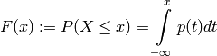
given the probability mass function  .
For sampling, the inverse cumulative distribution function
.
For sampling, the inverse cumulative distribution function  (i-cdf)
is especially interesting. If a closed form representation exists, one can sample
the uniform distribution (which usually is relatively easy) in the i-cdf’s
domain
(i-cdf)
is especially interesting. If a closed form representation exists, one can sample
the uniform distribution (which usually is relatively easy) in the i-cdf’s
domain ![y \in [0,1]](_images/math/fd49baf2ab76d48a4af3e82f0c7aa40e6f65a559.png) and then use the i-cdf to retrieve samples distributed
according to its probability distribution:
and then use the i-cdf to retrieve samples distributed
according to its probability distribution:
- Draw
![u \sim \mathcal{U}^{[0,1]}](_images/math/5f04f9ba36222b130f223cc975924e787a7d7ff1.png)
- Obtain a sample

The numpy.random package contains several functions to sample directly from the most prominent distributions. Unfortunately, the inverse cdf does not always exist, which makes more complex methods inevitable.
3.2. Sampling from arbitrary distributions
The target sample distribution may not always be known (e.g. it can be determined by measurements from a source with unknown distribution) or a closed form representation of the i-cdf may could not be available. In this case, a more elaborate mechanism has to be made use of (which, as always, comes with the cost of less efficient computation).
3.2.1. Rejection sampling
This is a relatively simple but often inefficient sampling scheme. A proposal
distribution  is required as well as a scaling constant
  .
The proposal distribution can have any shape, but it must be guaranteed that
.
The proposal distribution can have any shape, but it must be guaranteed that

with the target distribution. To find any tuple  that
fullfills the above equation is often not very hard find. However, as described
later, the larger the scaling, the less efficient the algorithm becomes and
finding an acceptable tuple may be difficult.
that
fullfills the above equation is often not very hard find. However, as described
later, the larger the scaling, the less efficient the algorithm becomes and
finding an acceptable tuple may be difficult.
The algorithm can then be laid out:
Iterate, until
 accepted samples have been generated
- Sample from the proposal

- Sample from the uniform distribution
![u \sim U^{[0,1]}](_images/math/411270df92bd8fdf7988c395f91b5ab98742da9d.png)
- Accept the sample
 , if
, if  .
Reject it otherwise.
.
Reject it otherwise.
- Sample from the proposal
As it can be seen from the algorithm, a sample has to be obtained from the
distribution , hence a proposal distribution should
be chosen that is relatively easy to sample. A sample is accepted,
iff , thus the probability
that a sample is accepted is proportional to  . If the
proposal and target distributions don’t match well, the scaling has to be large
which introduces massive performance issues.
. If the
proposal and target distributions don’t match well, the scaling has to be large
which introduces massive performance issues.
3.3. Interfaces
- ailib.sampling.rouletteWheelN(data, weights, numSamples)
Return samples drawn from a discrete distribution.
Parameters: - data ([a]) – List of tokens.
- weights ([float]) – Weights of tokens.
- numSamples (int) – Number of samples to draw.
Returns: numSamples samples drawn from data according to their weights.
- ailib.sampling.rouletteWheel(data, weights)
Return a sample drawn from a discrete distribution.
Parameters: - data ([a]) – List of tokens.
- weights ([float]) – Weights of tokens.
Returns: Generator object for samples drawn from data according to their weights.
- ailib.sampling.rejectionSamplerN(qSampler, qDist, pDist, N, M)
Draw samples from a distribution, given its probability density function.
This sampler can be used, if the probability density function of the target distribution is known, but there’s no direct sampling approach (e.g. the inverse cdf is not known).
Parameters: - qSampler (a) – Sampling function of the proposal distribution.
- qDist ((Num b) => a -> b) – Probability density function of the proposal distribution.
- pDist ((Num b) => a -> b) – Probability density function of the target distribution.
- N (int) – Number of samples.
- M (float) – Scale parameter.
Returns: N samples, distributed according to the probability density of the target distribution pDist.
- ailib.sampling.rejectionSampler(qSampler, qDist, pDist, M)
Draw samples from a distribution, given its probability density function.
This sampler can be used, if the probability density function of the target distribution is known, but there’s no direct sampling approach (e.g. the inverse cdf is not known).
Parameters: - qSampler (a) – Sampling function of the proposal distribution.
- qDist ((Num b) => a -> b) – Probability density function of the proposal distribution.
- pDist ((Num b) => a -> b) – Probability density function of the target distribution.
- M (float) – Scale parameter.
Returns: Generator for samples, distributed according to the probability density of the target distribution pDist.
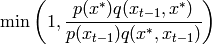
- ailib.sampling.metropolisHastingsSampler(qSampler, qDist, pDist, x0=0.0)
Draw samples from a distribution.
Parameters: - qSampler (a -> a) – Sampling function of the proposal distribution.
- qDist ((Num b) => a -> a -> b) – Probability density function of the proposal distribution.
- pDist ((Num b) => a -> b) – Probability density function of the target distribution.
- x0 (a) – Initial value
Returns: Generator object for samples, distributed according to the target distribution pDist.
The proposal is
- ailib.sampling.metropolisSampler(qSampler, qDist, pDist, x0=0.0)
Draw samples from a distribution.
Parameters: - qSampler (a -> a) – Sampling function of the proposal distribution.
- pDist ((Num b) => a -> b) – Probability density function of the target distribution.
- x0 (a) – Initial value
Returns: numSamples samples, distributed according to the target distribution pDist.
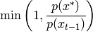
The metropolis sampler assumes a symmetric proposal, i.e.
This reduces the proposal to