4.3.1. Linear Regression
4.3.1.1. Generalized linear models
Given an input vector ![\vec{x} = \left[ x_1, x_2, \dots, x_p \right]^T](_images/math/1b750500f0010b3f0fa422d7bdb24d49ca7c25e2.png) and coefficients
and coefficients
![\vec{\beta} = \left[ \beta_0, \beta_1, \beta_2, \dots, \beta_p \right]^T](_images/math/983c0de1774b0acac8aaa16a35fca1517c3accb6.png) .
A generalized linear model is the function of the form:
.
A generalized linear model is the function of the form:
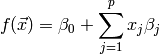
This notation describes any function with linear dependence on the parameters  .
For example, a polynomial can be written as
.
For example, a polynomial can be written as
![f(\vec{x}) = \beta_0 + \sum\limits_{j=1}^p x_j \beta_j \quad \text{with } \vec{x} = \left[ x, x^2, \dots, x^p \right]](_images/math/f30b95bba99ac9f1dbfaa72a9e7ed2f742b68131.png)
The fitting problem focuses on finding the optimal parameters of the function  for
for  given training pairs
  , with
  being the target output.
In this context, optimal means that the allocation of
being the target output.
In this context, optimal means that the allocation of  needs to minimize the sum of squared residuals:
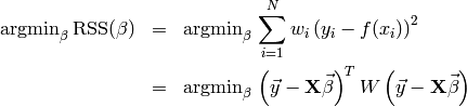
The lower equation is just there to get rid of the sum. The matrix  holds all the training input vectors (size
  ), the matrix
  is a diagonal matrix
with
is a diagonal matrix
with  .
.
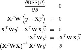
As known from basic analysis, the extremal points (here the minimum) can be found by setting the
function derivative to zero. In the problem setting, the training samples are fixed and the
optimization goes for the parameters, thus we’re interested in the derivative w.r.t the parameters 
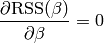
The nice property of generalized linear models is that this derivation can easily be determined:
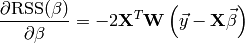
Putting the above ideas toghether yields the closed form solution of the fitting problem:
The generalization to  outputs can be done, if
  is written as (
 )-matrix with each row a set
of output values. Then the coefficients are computed the same way as above,
becoming a (
)-matrix with each row a set
of output values. Then the coefficients are computed the same way as above,
becoming a ( ) matrix. Note that the outputs are independent of each
other, thus solving the system with multiple outputs it is equivalent to solving the system
once for each single output. [ESLII]
) matrix. Note that the outputs are independent of each
other, thus solving the system with multiple outputs it is equivalent to solving the system
once for each single output. [ESLII]
4.3.1.1.1. Ridge regression
The above described least squares routine may lead to severe overfitting problems. The generalization error might even decrease, if some of the coefficients are set to zero.
Instead of removing a coefficient subset, the ridge regression introduces a penalty on the size of the coefficients. The idea is that the sum of squared coefficients may not exceed a threshold. This forces less significant coefficients to vanish while the most influencing ones shouldn’t be changed too heavily. Using lagrange multipliers, the optimization problem is stated the following way:
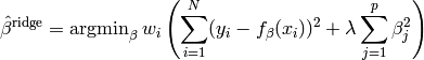
The parameter  is introduced to control the amount of shrinkage.
The larger
is introduced to control the amount of shrinkage.
The larger  , the more the coefficients are constrained. For
  ,
the problem becomes identical to the ordinary least squares.
,
the problem becomes identical to the ordinary least squares.
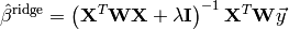
As for ordinary least squares, the sum of squared residuals can be formulated

and by its derivation with respect to , the closed form solution is found:
4.3.1.2. Interfaces
- class ailib.fitting.LinearModel(lambda_=0.0)
Generalized linear model base class.
Although possible, it’s generally not a good idea to use this class directly. Instead, use a derived classes, such as BasisRegression.
Subclasses are required to write the coeff member after fitting. Otherwise some routine calls may fail or produce wrong results.
Parameter: lambda (float) – Shrinkage factor. - err(x, y)
- Squared residual.
- eval(x)
Evaluate the model at data point x.
The last computed coefficients are used.
Todo
This routine doesn’t work, if x is a scipy.matrix
Parameter: x ([float]) – (p+1) Basis inputs. Returns: Model output.
- fit(data, labels, weights=None)
Fit the model to some training data.
Parameters: - data ([a]) – Training inputs.
- labels ([b]) – Training labels.
- weights ([float]) – Sample weights.
Returns: self
- numCoeff()
- Number of basis values.
- numOutput()
- Number of output values.
- class ailib.fitting.BasisRegression(lambda_=0.0)
Least squares regression with arbitrary basis input.
This class allows to use arbitrary basis functions. The resulting model is
f(x) = c0*b0(x) + c1*b1(x) + c2*b2(x) + c3*b3(x) + ...
with b0(x) := 1.0
The basis functions can be registered using the addBasis method. Any function can be used, the only requirement is that the type of its only argument is the same type as the model input x (see below).
Parameter: lambda (float) – Shrinkage factor. - addBasis(b)
Add a basis function.
Parameter: b ((Num b) :: a -> b) – Basis function.
- eval(x)
- Evaluate the model at data point x.
- fit(data, labels, weights=None)
Fit the model to some training data.
Parameters: - data (a) – Training inputs.
- labels (b) – Training labels.
- weights ([float]) – Sample weights.
Returns: self
- class ailib.fitting.PolynomialRegression(deg, lambda_=0.0)
Polynomial regression.
For fitting a polynomial f(x) = c0 + c1*x + c2*x**2 + c3*x**3 + ...
Parameters: - deg (int) – Degree of polynomial (largest exponent)
- lambda (float) – Shrinkage factor.
4.3.1.3. Examples
Let’s define a toy function that generates some samples and fits a polynom using them.
def polyEst(lo, hi, numSamples, sigma, deg, l=0.0):

    # Setting up the true polynomial and estimator
    poly = lambda x: 1.0 + 2.0*x  + 3.0*x**2 + 0.5*x**3 + 0.25*x**4 + 0.125*x**5
    est = ailib.fitting.PolynomialRegression(deg, lambda_=l)

    # Generate samples from the polynomial
    x = [lo + (hi - lo) * random.random() for i in range(numSamples)]
    y = [poly(i) + random.gauss(0.0, sigma) for i in x]

    # Fit the estimator to the samples
    est.fit(x,y)
    return est, (x,y)

# y = exp(a0*x0) * exp(a1*x1) * exp(a2*x2)
# ln(y) = ln( ... ) = ln(exp(a0*x0)) + ln(exp(a1*x1) + ln(exp(a2*x2)) = a0*x0 + a1*x1 + a2*x2
>>> print est(0.0, 1.0, 1000, 1.0, 5)
Poly(1.06417448201 * x**0 + 1.90233085087 * x**1 + -1.80439247299 * x**2 + 25.2719255838 * x**3 + -38.4765407136 * x**4 + 19.0506853189 * x**5)